RNN in Time Series Forecasting
Topic: Deep Learning · Time Series · Reading time: ~15 min
Contents
1) Introduction: Why Recurrence Matters
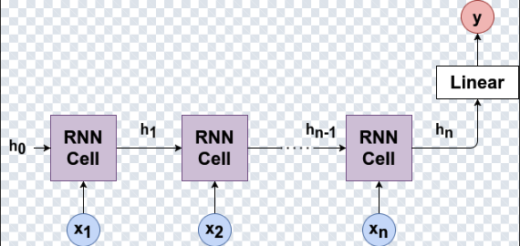
Time series are sequential: order matters, and the past influences the future. Classical statistical models (e.g., autoregressive processes) encode this dependency with fixed lag structures. Neural networks need a different mechanism to carry information forward in time.
Recurrent Neural Networks (RNNs) address this by introducing an internal state that evolves as the model reads the sequence.
This is why RNNs are called “recurrent.”
As each new value in the sequence arrives, the network updates its hidden state by combining the current input with information accumulated from previous timesteps.
This principle underlies all recurrent architectures: vanilla RNNs, GRUs, and LSTMs.
2) RNNs as Nonlinear Autoregressive Models
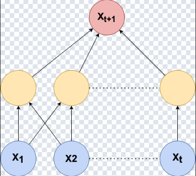
From a time-series perspective, an RNN can be viewed as a nonlinear autoregressive model with learned memory.
Classical AR intuition:
x_{t+1} = f(x_t, x_{t-1}, ..., x_{t-p})An RNN replaces the explicit lag order p with a hidden state that summarizes the past:
h_t = f(h_{t-1}, x_t)
x̂_{t+1} = g(h_t)
The hidden state acts as an adaptive compression of history—the model learns what information to keep, rather than forcing you to choose a fixed lookback window in advance.
Key limitation: vanishing gradients
Vanilla RNNs often struggle to learn long-term dependencies. During backpropagation through time, gradients can shrink exponentially (vanishing gradients), so information from far in the past barely influences learning. This is the main reason gated architectures were introduced.
3) GRU: Selective Memory
Gated Recurrent Units (GRUs) mitigate the vanishing gradient problem by using gates that control what to remember and what to forget—while remaining simpler than LSTMs.
GRUs use two gates:
- Reset gate: controls how much past information to ignore.
- Update gate: controls how much past information to keep versus how much to replace.
The defining operation of a GRU is a smooth interpolation between old and new information:
h_t = (1 - z_t) ⊙ h_{t-1} + z_t ⊙ h̃_t
Intuitively, the update gate z_t behaves like a soft switch: it helps the model preserve useful memory and update only when needed.
This often leads to fast training and strong performance in forecasting tasks.
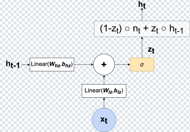
z_t blends the previous hidden state with the candidate state to produce h_t.
4) Mathematical Insight (Compact View)
If you want a compact mathematical picture, here are the core equations (useful to connect the intuition to the formalism).
GRU (summary)
z_t = σ(W_z x_t + U_z h_{t-1} + b_z)
r_t = σ(W_r x_t + U_r h_{t-1} + b_r)
h̃_t = tanh(W_h x_t + U_h (r_t ⊙ h_{t-1}) + b_h)
h_t = (1 - z_t) ⊙ h_{t-1} + z_t ⊙ h̃_t
The update gate helps prevent overwriting useful memory, which stabilizes learning over time.
5) LSTM: Explicit Long-Term Memory
Long Short-Term Memory (LSTM) networks introduce a dedicated cell state c_t
that acts like a long-term memory highway. This gives LSTMs finer control over what is stored, forgotten, and exposed—at the
cost of more parameters and computation.
LSTMs use three gates:
- Forget gate: what to discard.
- Input gate: what to write into memory.
- Output gate: what to expose as the hidden state.
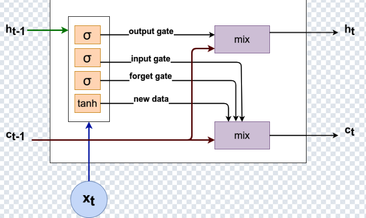
c_t (long-term memory) and the hidden state h_t (exposed output).
Compact LSTM equations
f_t = σ(W_f x_t + U_f h_{t-1} + b_f)
i_t = σ(W_i x_t + U_i h_{t-1} + b_i)
o_t = σ(W_o x_t + U_o h_{t-1} + b_o)
c_t = f_t ⊙ c_{t-1} + i_t ⊙ c̃_t
h_t = o_t ⊙ tanh(c_t)
In practice, LSTMs can shine when very long dependencies matter (long seasonality, long trends, structural changes), but GRUs are often an excellent default baseline.
6) RNN vs GRU vs LSTM (Forecasting Perspective)
| Model | Memory | Complexity | Best use case |
|---|---|---|---|
| RNN | Hidden state only | Low | Short sequences |
| GRU | Gated hidden state | Medium | General forecasting (great default) |
| LSTM | Hidden + cell state | High | Very long dependencies |
Rule of thumb: Start with a GRU. Switch to LSTM if you truly need stronger long-term memory.
7) Conclusion
Recurrent architectures are a natural fit for time series forecasting: they implement state recurrence that carries information from past to present. Vanilla RNNs are limited on long sequences, which motivates the use of GRUs and LSTMs.
GRUs often provide an excellent balance between stability, performance, and compute. LSTMs remain valuable when very long-range structure is critical.
References
- Ivan Gridin, Time Series Forecasting Using Deep Learning.
- Gated Recurrent Unit, ScienceDirect: https://www.sciencedirect.com/topics/computer-science/gated-recurrent-unit