ARCH and GARCH Models – Salem Nkunda Nyisingize

📅 March 2026 ⏱️ ~10 min read 🏷️ Time Series • Volatility • Financial Econometrics

A quiet seismic record can suddenly erupt into violent activity. For a while, the signal may look almost calm, only to be followed by a burst of tremors and then another quiet interval. Financial time series often behave in a remarkably similar way. Daily returns may fluctuate mildly for months, then experience a storm of extreme movements. This alternating pattern of calm and turbulence is one of the main reasons why classical constant-variance models are often not enough.

In such situations, the series may still resemble white noise in its mean behavior, yet its variability changes over time. This phenomenon is known as volatility clustering: large changes tend to be followed by large changes, and small changes tend to be followed by small changes. ARCH and GARCH models were developed precisely to describe this kind of dynamic variance.

1) When White Noise Is Not Really “Stable”

In many applications, the innovations $a t$ may appear uncorrelated, but their magnitude is clearly not constant across time. A classic example is the series of Dow Jones daily returns from October 1, 1928 to December 31, 2010 (dataset $dow.rate$ in Applied Time Series Analysis). Certain periods, especially the 1930s, display sustained turbulence, while isolated extremes stand out around events such as the 1929 crash and Black Monday on October 19, 1987.

Important point: uncorrelated does not mean normally distributed. Correlation is only a measure of linear dependence. A process may have zero autocorrelation and still exhibit strong nonlinear dependence through its changing variance.

To model this, we focus on the conditional variance of the innovation process.

σ 2 t|t-1 = E(a t 2 | a t-k, k = 1, 2, ...)

This quantity represents the expected squared innovation given the past. In standard white noise, it would be constant. In ARCH/GARCH models, it evolves through time.

2) ARCH(1): The Basic Idea

The simplest ARCH model is built from

a t = σ t|t-1 ε t

where $ε t$ is an i.i.d. sequence with mean 0 and variance 1, independent of the past. The conditional variance is defined by

σ 2 t|t-1 = α 0 + α 1 a t-1 2, 0 \leq α 1 < 1

In words: today’s volatility depends on yesterday’s squared shock. A large shock yesterday increases the conditional variance today.

3) Why This Is Indeed the Conditional Variance

Starting from

a t = σ t|t-1 ε t

we get

a t 2 = σ 2 t|t-1 ε t 2

Taking conditional expectation with respect to the past,

E(a t 2 | a t-k, k = 1, 2, ...) = σ 2 t|t-1 E(ε t 2 | a t-k, k = 1, 2, ...)

Since $ε t$ is independent of the past and has unit variance,

E(ε t 2) = 1

therefore

E(a t 2 | a t-k, k = 1, 2, ...) = σ 2 t|t-1

This confirms that the model really specifies the conditional variance of the process.

4) Squared Innovations Behave Like an AR Process

Rearranging the ARCH(1) equation gives

a t 2 - (α 0 + α 1 a t-1 2) = σ 2 t|t-1 (ε t 2 - 1)

so we can write

a t 2 = α 0 + α 1 a t-1 2 + w t

where

w t = σ 2 t|t-1 (ε t 2 - 1)

This is one of the key insights behind ARCH models: although $a t$ itself may be uncorrelated, $a t 2$ can display serial dependence. That is why the ACF of squared residuals is central in volatility analysis.

5) The ARCH(q) Model

ARCH(1) is only the first step. More generally, an ARCH(q) model allows several past squared shocks to affect current variance:

a t = σ t|t-1 ε t σ 2 t|t-1 = α 0 + α 1 a t-1 2 + α 2 a t-2 2 + ... + α q a t-q 2

Equivalently, the squared process can be written as

a t 2 = α 0 + α 1 a t-1 2 + α 2 a t-2 2 + ... + α q a t-q 2 + w t

6) The GARCH(p, q) Model

The ARCH model is generalized by allowing past conditional variances to influence the present one. This leads to the GARCH model:

a t = σ t|t-1 ε t σ 2 t|t-1 = α 0 + β 1 σ 2 t-1|t-2 + ... + β p σ 2 t-p|t-p-1 + α 1 a t-1 2 + ... + α q a t-q 2

GARCH models are especially useful because they capture both short-term reactions to shocks and longer-term persistence in volatility.

7) Unconditional Variance

For a stationary GARCH process, the unconditional variance is

σ 2 a = α 0 / [1 - (α 1 + β 1) - ... - (α m + β m)]

where the denominator reflects the total persistence of past squared shocks and past variances. The closer this total is to 1, the more persistent the volatility.

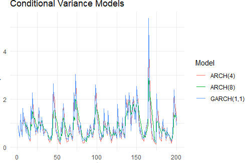
8) Three Concrete Examples

ARCH(4)

σ 2 t|t-1 = 0.1 + 0.36a t-1 2 + 0.27a t-2 2 + 0.18a t-3 2 + 0.09a t-4 2

ARCH(8)

σ 2 t|t-1 = 0.1 + 0.2a t-1 2 + 0.175a t-2 2 + 0.15a t-3 2 + 0.125a t-4 2 + 0.1a t-5 2 + 0.075a t-6 2 + 0.05a t-7 2 + 0.025a t-8 2

GARCH(1,1)

σ 2 t|t-1 = 0.1 + 0.45a t-1 2 + 0.45σ 2 t-1|t-2

Interpretation: the two ARCH models react only to past squared shocks, while the GARCH(1,1) model also remembers its own past volatility. That extra memory is often what makes GARCH more realistic for financial series.

9) Visual Interpretation

When exploring simulated or estimated volatility curves, one notices an increasing tendency for extreme changes in conditional variability as persistence grows. In ARCH(1), as $α 1 \to 1$ , large past shocks exert stronger and longer-lasting effects on future variance. In GARCH models, this persistence becomes even more visible because past variance itself re-enters the recursion.

The practical consequence is intuitive: volatility stops looking like isolated spikes and begins to appear in clusters. That is exactly what one often sees in finance, seismic data, and other systems characterized by intermittent bursts of intensity.

Comparison of ARCH(4), ARCH(8), and GARCH(1,1) conditional variance models. The GARCH curve typically shows greater persistence in volatility.

10) Conclusion

ARCH and GARCH models extend classical time series analysis by recognizing that uncertainty is not constant through time. Even when returns or residuals appear uncorrelated in the mean, their variance may reveal a rich and persistent structure.

This is why volatility modeling occupies such an important place in modern econometrics. It helps us understand why crises come in waves, why turbulence seems to have memory, and why the study of conditional variance is essential whenever calm and instability alternate in a time series.

Reference

Applied Time Series Analysis